
|
|
The Normal Distribution
The Normal Distribution is a continuous variable distribution which occurs very frequently. It models, for example, the distribution of heights of people, the weights of similar animals, and measurements on machine produced items.
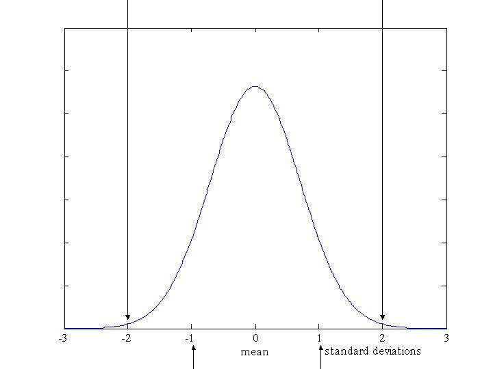
For ALL normal distributions:
![]() the distribution is symmetrical about the mean, which is also the median and the mode;
the distribution is symmetrical about the mean, which is also the median and the mode;
![]() approximately 95% of values fall within 2 standard deviations of the mean;
approximately 95% of values fall within 2 standard deviations of the mean;
|
![]() 68% (approximately two thirds) of values fall within 1 standard deviation of the mean;
68% (approximately two thirds) of values fall within 1 standard deviation of the mean;
![]() approximately 99.5% of values lie within 3 standard deviations of the mean.
approximately 99.5% of values lie within 3 standard deviations of the mean.
When doing any question involving the Normal Distribution it is recommended that you draw a small sketch first.
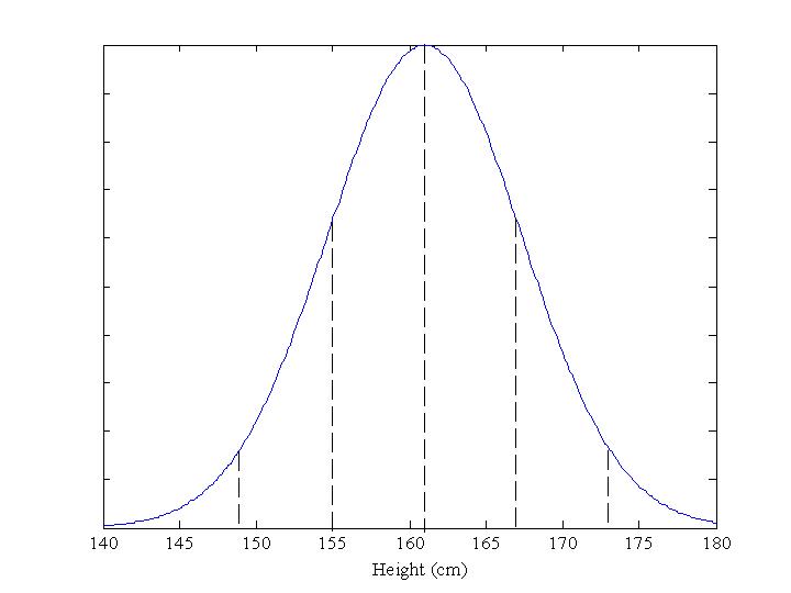
The heights of British women follow a Normal Distribution with a mean of 161cm and a standard deviation of 6cm. Here's the graph of the distribution:
|
What proportion will be more than 161cm in height? Answer: 50%
What proportion be between 155cm and 167cm tall? Answer: 68%.
What proportion will be more than 173cm tall? Answer: 2·5%
(Since 95% are between 149cm and 173cm, 5% will be either shorter or taller. As the distribution is symmetric, half of them will be taller.)
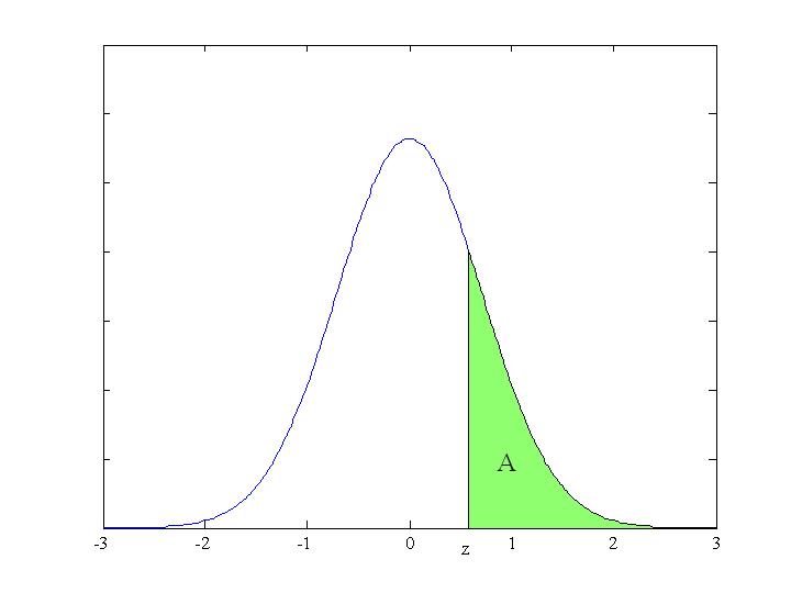
Normal Distribution tables use the standard normal distribution with a mean of 0 and a standard deviation of 1.
The table shows the values of z which measures the distance from the mean in standard deviations.
|
The shaded area, A, gives the probability that z is greater than the given value.
![]() Z
Z ![]() .00
.00 ![]() .01
.01 ![]() .02
.02 ![]() .03
.03![]() .04
.04
0.0 0.5000 0.4960 0.4920 0.4880 0.4840
0.1 0.4602 0.4562 0.4522 0.4483 0.4443
0.2 0.4207 0.4168 0.4129 0.4090 0.4052
0.3 0.3821 0.3783 0.3745 0.3707 0.3669
0.4 0.3446 0.3409 0.3372 0.3336 0.3300
0.5 0.3085 0.3050 0.3015 0.2981 0.2946
0.6 0.2743 0.2709 0.2676 0.2643 0.2611
0.7 0.2420 0.2389 0.2358 0.2327 0.2296
0.8 0.2119 0.2090 0.2061 0.2033 0.2005
0.9 0.1841 0.1814 0.1788 0.1762 0.1736
1.0 0.1587 0.1562 0.1539 0.1515 0.1492
This is only a small extract.
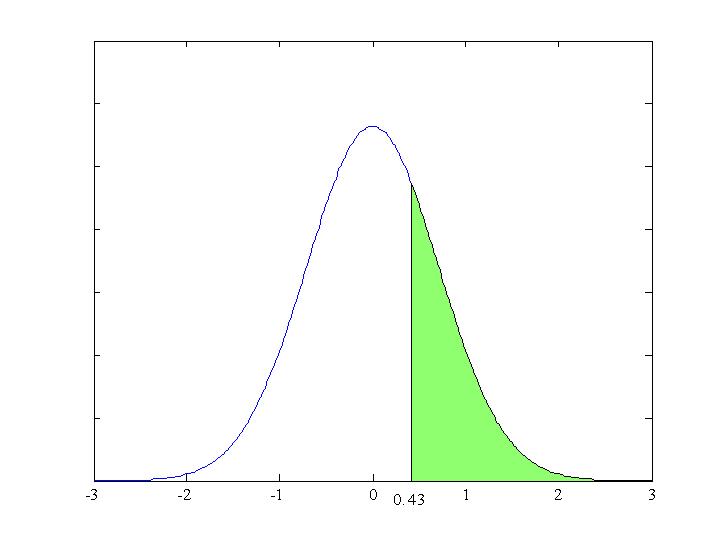
To find ![]() means "find the probability that z is greater than 0.43". The graph representing this is shown below.
means "find the probability that z is greater than 0.43". The graph representing this is shown below.
|
Look along the 0.4 row and under the .03 column. The number you will find is 0.3336 which is the required probability.
To find the probability that z is a value less than 0·43, we take 0·3336 from 1.
![]() .
.
Sometimes we want to know the probability that z is a value between 0 and another number, e.g. 0 and 0·43, as shown in the graph below.
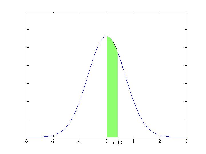
|
We know ![]() and that the area to the right of 0 (shaded ) equals 0·5,
and that the area to the right of 0 (shaded ) equals 0·5,
so ![]() .
.
The probability density function which describes the normal distribution is given by
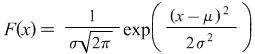
where ![]() is the standard deviation and
is the standard deviation and ![]() is the mean.
is the mean.
The moment generating function of the normal distribution is
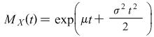 .
.